Spark Execution Model

The driver and the DAG

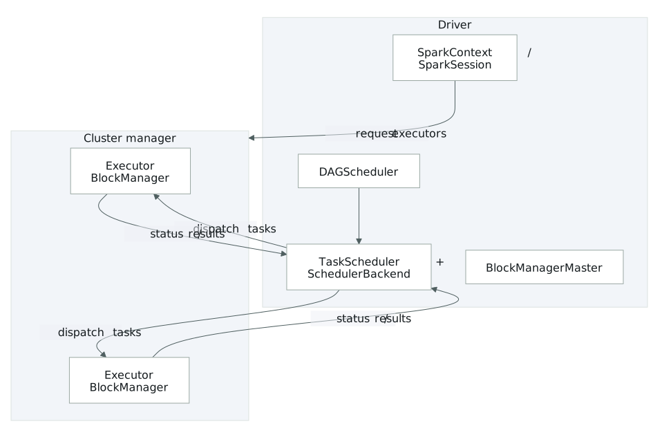
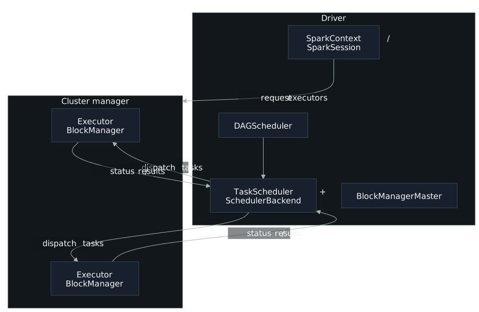
The Driver is the process "in the driver seat" of a Spark application: it controls execution and maintains all state of the cluster, including the state and tasks of the executors, and it interfaces with the cluster manager to obtain physical resources and launch executors^[1]. It runs as a single JVM process (on the submission machine in client mode, or on a dedicated cluster node in cluster mode), and if it dies, the application dies with it^[2].

As application code executes, the Driver incrementally builds a logical DAG of RDD/DataFrame transformations. Because Spark is lazy, nothing actually computes until an action is called; only then does the Driver convert the logical DAG into a physical plan, cut it into stages at wide-dependency (shuffle) boundaries, break each stage into one task per partition, and take on the scheduler's job: talking to the cluster resource manager to request executors, handing out tasks, tracking their progress, and resubmitting tasks whose executor died^[2:1].

Three components live only on the Driver:

• The DAGScheduler reads RDD lineage, decides stage boundaries at wide dependencies, emits per-partition TaskSets, tracks lineage so lost partitions can be recomputed, and reacts dynamically to stage completions rather than pre-scheduling the whole DAG up front; it also declares a job failed if a stage can't make progress^[2:2].
• The BlockManagerMaster is the Driver-side counterpart to each executor's own BlockManager. It keeps the global map of block locations (RDD partitions, shuffle files, broadcast variables) across the whole cluster, so a task's local BlockManager knows where to fetch a remote block from^[2:3].
• The SparkContext (wrapped today by SparkSession) is the entry point that lets the Driver talk to the cluster manager, request executors, create RDDs, and manage shared variables. It's instantiated once per application and lives for the application's whole lifetime^[2:4].

Executors, by contrast, hold no cluster-wide state: they only run the tasks assigned to them and report back success, failure, and results^[1:1]. The split even shows up at the configuration level: spark.driver.host/spark.driver.port and spark.driver.blockManager.port are Driver-specific listening endpoints, distinct from the equivalent executor settings^[3].

A Spark job corresponds to one action, and each job breaks down into a series of stages: how many depends on how many shuffle operations need to happen^[1:2]. A stage is a group of tasks that can execute together to compute the same operation across machines: work one executor can do without communicating with other executors or the Driver. A new stage begins whenever data has to move across the network, that is, at a shuffle^[4]. Wide transformations, such as groupByKey, join, and sortByKey, create ShuffleDependency objects, and it's these ShuffleDependencys that mark the stage boundary; several narrow transformations can be grouped into the same stage^[4:1]. Within a stage, the number of tasks equals the number of partitions in that stage's output RDD: one task per partition, each running the same code on a different slice of data^[4:2].

The rule is always "a shuffle dependency creates the boundary," and that isn't limited to an explicit .repartition() or .groupBy() call: sortByKey/sortBy on an RDD is itself a wide transformation, not just groupByKey-style aggregations^[4:3]. The original Spark paper defines stage boundaries generically, as the shuffle operations required for wide dependencies, or already-computed partitions that can short-circuit the computation of a parent RDD^[5]. A wide dependency of any kind is what matters, not a specific API call.

That wide/narrow split has a formal definition behind it. Conceptually, a narrow transformation is one where each partition in the child RDD has simple, finite dependencies on partitions in the parent RDD, determinable at design time regardless of the values of the records; narrow dependencies allow pipelined, one-node execution, while wide dependencies require data from all parent partitions to be shuffled across nodes^[5:1]. The formal 2012 definition is stated from the parent's side rather than the child's: a transformation is narrow if "each partition of the parent RDD is used by at most one partition of the child RDD," and wide if "multiple child partitions may depend on" a given parent partition^[4:4]. That parent-centric framing is more precise, because Spark's DAG scheduler builds the execution plan backward from the action to the input RDD, and it correctly rules out the case of one parent partition feeding multiple children under "narrow"^[4:5].

mapPartitions is narrow under this definition: each child partition depends on exactly one parent partition, the same as map and filter^[4:6]. coalesce is narrow too, even though it changes the number of partitions and a child partition can depend on multiple parent partitions: the rule only requires that each parent partition be used by at most one child partition, and which parent partitions merge into which child is fixed at design time, independent of the data's values. That holds specifically when coalesce reduces the partition count; when it increases the count, it behaves like repartition, a shuffle^[4:7].

Pipelining is what makes narrow dependencies pay off. Spark performs as many steps as possible in one pass before writing data to memory or disk: any sequence of operations that feed data directly into each other, without moving data across nodes, collapses into a single stage of tasks that execute all the operations together. map → filter → map becomes one stage whose tasks read each record and pass it through all three operations in sequence, rather than materializing intermediate results after each step; the same collapsing happens for a DataFrame/SQL computation doing select → filter → select^[1:3]. The original paper phrases the mechanism at the scheduler level: to run an action, Spark builds stages at wide dependencies and pipelines narrow transformations inside each stage^[5:2].

Two more components take over once a job's stages exist. The DAGScheduler is Spark's high-level scheduling layer: it takes RDD dependencies, builds a DAG of stages for each job, determines where each task should run, and passes that to the TaskScheduler^[4:8]. The TaskScheduler takes it from there and stops thinking in terms of RDDs, lineage, or shuffles: only machines and slots. It works with the SchedulerBackend to request executors, assigns tasks to executors while respecting data-locality preferences, and retries failed tasks, including resubmitting a task elsewhere if its executor died^[2:5]. The TaskScheduler doesn't launch tasks directly; it hands them to the SchedulerBackend, the layer that actually talks to the cluster manager to request, launch, and kill executors^[2:6].

Finally, at the RDD API level spark.default.parallelism sets the default partition count for distributed shuffle operations like reduceByKey and join. It defaults to the largest number of partitions in the parent RDD, and for operations with no parent RDD, such as parallelize, the default depends on the cluster manager^[3:1]. spark.sql.shuffle.partitions is the equivalent knob for the Spark SQL/DataFrame engine: it configures how many partitions Spark uses when shuffling data for joins or aggregations, and it defaults to 200 regardless of data size^[6], applying whenever a DataFrame/SQL operation triggers a shuffle: join, groupBy, distinct, orderBy, and so on^[7].

Reading stages and tasks

Once a job runs, stage and task counts show up directly in the Spark UI, and a worked example makes the mechanics concrete: a job that reads a range with 8 partitions produces a stage with 8 tasks; repartitioning to 6 and then 5 partitions produces stages with 6 and 5 tasks; a subsequent join shuffles into the default 200 shuffle partitions, producing a 200-task stage^[1:4]. The same logic explains stage counts for RDD pipelines: the chain filter → map → groupByKey → map → sortByKey → count produces three stages, bounded by the groupByKey and sortByKey operations, since both are wide^[4:9].

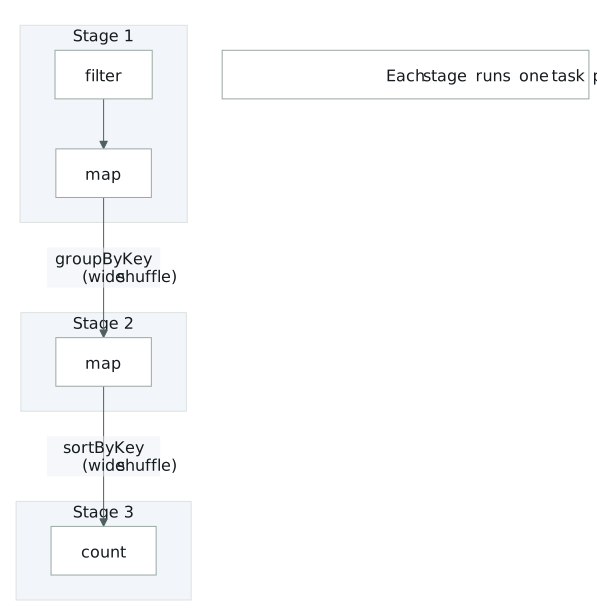
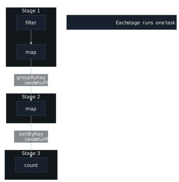
Pipelining is invisible to the application and only shows up in the Spark UI or logs, where multiple chained narrow operations appear collapsed into a single stage instead of one stage per operation^[1:5]. A related signal is the "skipped stage" marking: because Spark always writes shuffle output to stable storage regardless of any persist/checkpoint call, if the Driver reuses an RDD that was already shuffled, Spark can skip recomputing everything up to that shuffle and read the shuffle files directly. The Spark UI shows this as a skipped stage, not as an added boundary^[4:10].

When diagnosing partition counts, checking which knob is in play matters: spark.default.parallelism governs the legacy RDD API's shuffle and parallelize operations, while spark.sql.shuffle.partitions governs DataFrame/Dataset/SQL shuffles^[3:2]. Since Spark 3.0, Adaptive Query Execution (AQE) can also override the static spark.sql.shuffle.partitions value after the fact. It can coalesce many small post-shuffle partitions and split skewed ones at runtime, but only after the first shuffle has already happened, so it never explains the initial input partitioning^[7:1].

Why the boundary matters

Those stage boundaries aren't just a UI detail. Because a new stage begins only at a shuffle, the boundary is exactly where Spark pays the cost of moving data across the network. Everything inside a stage runs without that cost, pipelined on a single executor^[4:11].

That's also why the wide/narrow distinction determines whether pipelining is even possible: once a shuffle is required, downstream computation can't proceed until the shuffle completes, because the records landing on each partition may change as a result of it, so narrow transformations following a wide one belong to a new stage and can't be pipelined across that boundary^[4:12].

Whether pipelining happens can also depend on partitioning state Spark already knows about. Because Spark tracks how an RDD is already partitioned, the same operation can land in different stage boundaries depending on whether the input RDD already has a known partitioner: no shuffle, and hence no new stage, is needed if one is already in place^[4:13].

Checkpointing is a separate mechanism from all of this: it breaks RDD lineage and writes data to disk so later transformations start from a fresh, trimmed plan, rather than being pipelined against the original computation^[8].

The choice of shuffle-partition count matters for the same reason: there's no fixed formula for the right number, since it depends on data set size, number of cores, and available executor memory, and the default of 200 is called out as too high for smaller or streaming workloads, where it's better reduced toward the number of executor cores or less^[9]. coalesce's narrowness carries its own tradeoff: reducing partition count without a shuffle forces all upstream partitions in that stage to run at the coalesced parallelism level, which can be undesirable^[4:14].

On the scheduling side, Spark's scheduler is fully thread-safe and supports running multiple jobs concurrently if they're submitted from separate Driver threads, common when an application serves multiple concurrent requests over the network^[10]. By default Spark schedules jobs FIFO, which means an application running many jobs from multiple threads can have later jobs wait behind earlier ones unless a fairer policy is configured^[4:15].

Controlling parallelism and scheduling

Parallelism and scheduling are both tunable from here. When coalesce's single-parent-per-child constraint forces upstream parallelism lower than you want, repartition trades that limitation for an explicit shuffle, restoring full control over the resulting partition count^[4:16]. For the SQL/DataFrame engine, don't leave spark.sql.shuffle.partitions at its 200 default for small or streaming workloads: reduce it toward the number of executor cores or less, since the right value depends on data size, core count, and executor memory rather than a fixed rule^[9:1]. Where the data volume is unpredictable, Adaptive Query Execution (available since Spark 3.0) can take over after the fact: it coalesces many small post-shuffle partitions and splits skewed ones at runtime, though it only acts after the first shuffle has already happened and won't fix the initial input partitioning^[7:2].

For concurrent workloads, Spark also offers a fair scheduler as an alternative to the FIFO default, assigning tasks to concurrent jobs round-robin so each job gets a more even share of cluster resources^[4:17]; job pools and weights for finer-grained sharing are configured via spark.scheduler.mode=FAIR and the spark.scheduler.pool local property set on the submitting thread^[1:6]. Submitting jobs from separate Driver threads is what lets them run concurrently in the first place, rather than queuing behind each other^[10:1].

Sources

---

1. Spark: The Definitive Guide, Chambers & Zaharia, ch. 15–16 ↩︎ ↩︎ ↩︎ ↩︎ ↩︎ ↩︎ ↩︎

2. Anatomy of Spark Application ↩︎ ↩︎ ↩︎ ↩︎ ↩︎ ↩︎ ↩︎

3. Configuration — Spark ↩︎ ↩︎ ↩︎

4. High Performance Spark, 2nd Edition, Karau, Polak & Warren, ch. 2, 7–8 ↩︎ ↩︎ ↩︎ ↩︎ ↩︎ ↩︎ ↩︎ ↩︎ ↩︎ ↩︎ ↩︎ ↩︎ ↩︎ ↩︎ ↩︎ ↩︎ ↩︎ ↩︎

5. Resilient Distributed Datasets: A Fault-Tolerant Abstraction for In-Memory Cluster Computing ↩︎ ↩︎ ↩︎

6. Performance Tuning — Spark SQL, DataFrames and Datasets Guide ↩︎

7. Spark Partitions ↩︎ ↩︎ ↩︎

8. Spark Tips: Caching ↩︎

9. Learning Spark, 2nd Edition, Damji, Wenig, Das & Lee, ch. 7 ↩︎ ↩︎

10. Job Scheduling ↩︎ ↩︎