
Appearance
Partitioning
How partitions get sized and shuffled
Every partition Spark creates maps to exactly one task and one thread, which is why partition count and size drive so much of a job's performance[1]. The shuffle side of that is governed by a single default: spark.sql.shuffle.partitions, which defaults to 200 and applies to every join(), groupBy(), and aggregation regardless of how much data is actually moving[2][3].
Two operations reshape that layout, and they are not interchangeable. repartition(numPartitions) "return[s] a new RDD that has exactly numPartitions partitions"[4], and it earns that guarantee by always running a full hash shuffle: records are first spread across a temporary key space starting from a randomized position, seeded per-partition via XORShiftRandom, so upstream data ends up distributed evenly rather than clustered by its original layout. That feeds into a ShuffledRDD keyed by a HashPartitioner(numPartitions), then a CoalescedRDD lands it on exactly the requested count[4:1]. High Performance Spark puts the same mechanics more plainly: "repartition shuffles the RDD with a hash partitioner and the given number of partitions"[5]. That holds whether the new count is bigger or smaller than the current one. Repartition always performs the full shuffle just described, unlike coalesce[6].
coalesce, left at its default, does not shuffle at all: it's a narrow transformation where each output partition is simply the union of a fixed set of parent partitions decided at plan time, not routed by data values, so the stage's task count just drops to the coalesced number[5:1].
Neither repartition nor coalesce leaves behind a "known partitioner" the way partitionBy does[5:2]. That distinction is what Spark's join planner checks before it will skip a shuffle: it only does so when both sides already carry partitioner objects it can prove equal: matching partition counts for a HashPartitioner, matching range bounds for a RangePartitioner[5:3]. Its default shuffle hash join path makes the same point from the other side: it partitions the second dataset using the same partitioner as the first specifically so matching keys land together, which only lets a later shuffle be skipped when a shared, recognized partitioner is already in place beforehand[5:4].
There's also a hard ceiling on shuffle output, though it isn't something to design around: Spark's sort-based shuffle manager caps output partitions in serialized mode at PackedRecordPointer.MAXIMUM_PARTITION_ID + 1, roughly 16.8 million. The source code itself calls this "an extreme defensive programming measure," since no real shuffle comes remotely close to it[7].
Spotting a bad layout
That layout choice shows up as overhead in both directions once it's wrong: partitions that are too small flood the cluster with per-task scheduling overhead, while partitions that are too large create memory pressure and straggler tasks[1:1]. Learning Spark 2nd Edition frames the healthy target from the parallelism side rather than an absolute number: at least as many partitions as there are cores across the executors, so no core sits idle; more partitions than cores is fine as long as it doesn't drift into the small-partition overhead regime above[3:1].
A heavy filter is an easy-to-miss cause of imbalance: Spark doesn't shrink partition count when rows are filtered out, so 2,000 partitions holding 5% of the original rows just become 2,000 mostly-empty partitions[1:2].
To size shuffle partitions from a job's actual behavior rather than a guess, Cloudera's tuning guide takes a stage that already ran, computes the ratio between its Shuffle Spill (Memory) and Shuffle Spill (Disk) metrics, and multiplies total shuffle write by that ratio to estimate in-memory shuffle size, then rounds the resulting partition count up rather than down[8].
Skew specifically has documented, numeric detection thresholds under Adaptive Query Execution: a partition counts as skewed if it's larger than spark.sql.adaptive.skewJoin.skewedPartitionFactor (default 5.0) times the median partition size, and also larger than spark.sql.adaptive.skewJoin.skewedPartitionThresholdInBytes (default 256 MB)[2:1][9].
On the input side, spark.sql.files.maxPartitionBytes (defaulting to 128 MB) governs the target chunk size when Spark splits splittable file-based sources (CSV, JSON, line-delimited text) into input partitions, based on file size[1:3].
Where a bad layout costs you
Getting the partition count wrong costs more than the immediate slowdown suggests. Cloudera's tuning guide argues it's safer to over-provision partitions than to under-provision them, because Spark, unlike MapReduce, has low per-task startup overhead: "when in doubt, it's almost always better to err on the side of a larger number of tasks"[8:1].
Getting coalesce wrong costs more than the coalesce step itself: because it's narrow, it forces the entire upstream stage to run at the reduced parallelism, not just the final step[5:5]. Pushed too far (coalesce(1)), it kills parallelism outright, because coalesce doesn't rebalance data, it just stacks existing partitions together, so partitions that were uneven going in are still uneven coming out[1:4].
Once a shuffle stage has run, its output file count is locked in: you can't change it after the fact without inserting a stage barrier, such as writing to temporary storage or calling localCheckpoint(), between the shuffle and the write[10].
Join alignment has its own gotcha: calling repartition(n, col) with the same column and count on two separate DataFrames produces data that's plausibly laid out the same way, but it doesn't leave a trackable partitioner object behind. The planner has no recorded partitioner to compare, so it has no basis for treating the two sides as co-partitioned and skipping the shuffle at join time, even though the call sites look identical[5:6].
Fixing the layout
Fixing those costs starts with accepting there's no formula to look up. There's no single formula for the right spark.sql.shuffle.partitions value: it depends on data set size, core count, and executor memory, and comes down to trial and error[3:2]. As a starting point, Learning Spark notes the default of 200 is usually too high for small or streaming workloads, where it should be pulled down toward the executor core count[3:3].
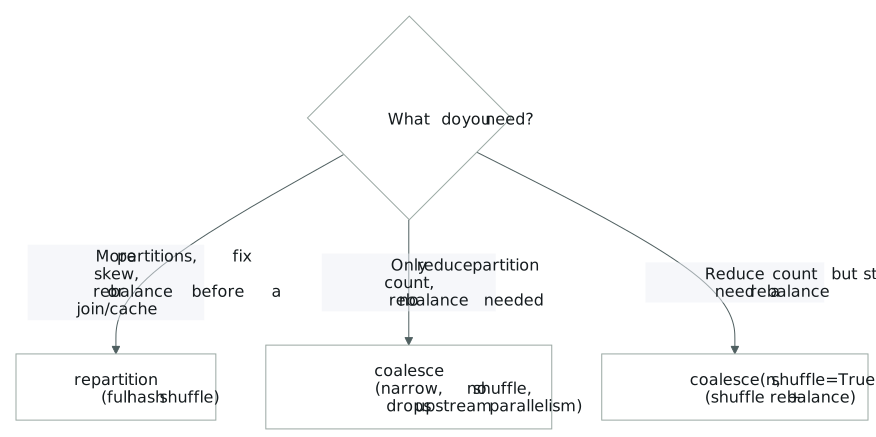
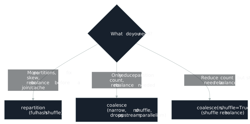
For the repartition-vs-coalesce decision itself: reach for coalesce first whenever you're only reducing partition count, since it merges partitions already on the same node without a shuffle[6:1]. Reach for repartition when you actually need the shuffle: increasing partition count, fixing a lopsided distribution, or preparing a DataFrame ahead of a join or a cache() call, where even parallelism is worth more than the shuffle cost[6:2]. High Performance Spark reduces this to a readability rule: use repartition when you want a shuffle, coalesce when you don't, rather than leaning on coalesce's shuffle toggle to blur the line[5:7]. There is a middle option, coalesce(n, shuffle=True), which behaves more like repartition, paying for a shuffle but getting real rebalancing on the way down[1:5]. coalesce() itself belongs at the tail of a pipeline, right before a write, purely to cut down output file count[1:6]; after a heavy filter has left partitions mostly empty, following up with repartition(100) (or similar) buys back real parallelism[1:7]. At the SQL layer, both directions have dedicated hints for controlling output partitioning directly: /*+ REPARTITION(n) */, /*+ REPARTITION(cols) */, /*+ REPARTITION_BY_RANGE(cols) */, and /*+ COALESCE(n) */[9:1].
Separate from the DataFrame .coalesce() call, Adaptive Query Execution has its own runtime coalescing behavior: spark.sql.adaptive.coalescePartitions.enabled (default true) merges small, contiguous post-shuffle partitions toward a target size at runtime, correcting over-partitioning without a manual .coalesce() call[9:2][1:8].
For skewed joins specifically, salting (adding a prefix to skewed keys so the same key is treated as several different keys, then adjusting the data distribution accordingly) was one of three manual approaches used before adaptive execution existed, alongside raising spark.sql.shuffle.partitions and raising the broadcast hash join threshold to push a sort-merge join toward a broadcast hash join instead. All three carry "lots of limitations" and require manual processing, which is exactly the gap AQE's skew-join optimization was built to close[11]. Where automatic detection isn't precise enough, Databricks' /*+ SKEW(...) */ hint names the skewed relation and column(s), and optionally the specific skewed key values, letting the planner target just those keys directly instead of relying on automatic detection[12].
For the join-alignment gotcha above, the mechanism that does reliably guarantee a shuffle can be skipped is storage-partitioned joins: both tables are physically bucketed identically at the catalog level, for example Iceberg tables created with matching PARTITIONED BY (bucket(...)) clauses. When Spark recognizes both sides report the same partitioning through SupportsReportPartitioning, it can drop the Exchange (shuffle) node entirely, or shuffle only one side. A plain DataFrame-level repartition(col) doesn't offer that guarantee, because it isn't backed by catalog-level partitioning metadata[9:3][2:2].