
Appearance
Adaptive Query Execution
What it is
The static Catalyst optimizer plans a query once, before execution, using cost estimates derived from static statistics: row counts, min/max, NDVs, or defaults when statistics are missing.[1] Adaptive Query Execution (AQE), shipped in Spark 3.0, instead re-optimizes the plan mid-execution using runtime statistics gathered from completed "query stages": the sections of a plan bounded by shuffle or broadcast exchange materialization points.[2] A shuffle or broadcast forces Spark to materialize its input before continuing, which makes it a natural checkpoint: once one or more leaf stages finish, AQE marks them complete, updates the logical plan with the real (not estimated) statistics, and reruns a selected set of logical and physical optimization rules (including AQE-specific rules such as partition coalescing and skew-join handling) before executing the next stages.[2:1]
Shuffle statistics only become available once a stage is fully materialized, not incrementally as individual map tasks finish. A stage's successor can only proceed once every parallel process producing that stage's output has completed, which is exactly why materialization points are the reoptimization opportunity: it's the moment when statistics on all of a stage's partitions are known and the next stage hasn't started yet.[2:2] AQE kicks off all leaf stages (the ones with no upstream dependency) first; as each one finishes, the framework marks it complete, updates the plan, and re-optimizes before launching whichever next stages now have all their children materialized. This execute→reoptimize→execute loop repeats (once per completed stage, not just once) until the whole query finishes, so the number of reoptimizations scales with how many shuffle/broadcast boundaries the plan has.[2:3] The Spark SQL config description for spark.sql.adaptive.enabled frames this the same way: AQE re-optimizes "the query plan in the middle of query execution, based on accurate runtime statistics."[3]
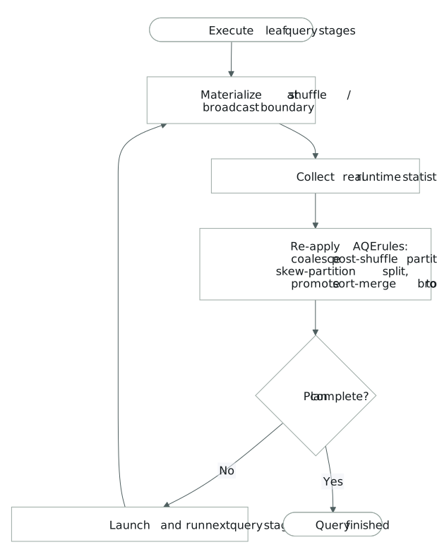
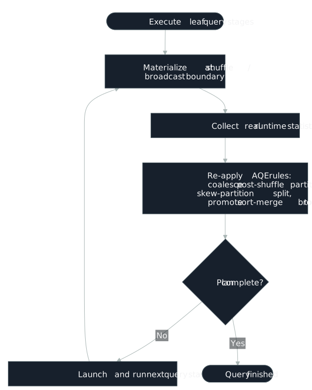
AQE re-optimizes three things the static optimizer cannot, because none of them are knowable before execution: the number of post-shuffle partitions (coalescing small partitions produced by wide transformations), the join strategy (converting a statically planned sort-merge join to a broadcast join once the actual materialized size of a join side is known), and skewed partitions in a shuffle join (splitting oversized partitions detected from shuffle file statistics).[2:4] High Performance Spark frames this as AQE using "runtime information about the data it is processing along with the target output to go beyond static optimizations," with partitioning and join strategy singled out as the two biggest areas it impacts.[4] AQE also performs empty-relation propagation, replacing subqueries that turn out to be empty (impossible joins, empty unions) with a dummy empty LocalRelation, again something only knowable once data is materialized.[4:1]
How it's detected
Because these are runtime decisions, none of them show up in a static explain() call; you have to run the query and check the Spark UI for the finalized, adapted plan.[4:2] The same caveat applies more broadly: since AQE adjusts plans at runtime, explain() might show one plan while the Spark UI shows a different one actually executed.[5]
What you're looking for in that adaptive plan are the specific runtime rewrites AQE can make:
- Partition coalescing. AQE combines adjacent small post-shuffle partitions into bigger ones by reading shuffle file statistics,[2:5] targeting
spark.sql.adaptive.advisoryPartitionSizeInBytes(default 64 MB).[6] In a worked example, five post-shuffle partitions where three are small get coalesced into one, cutting the final-aggregation task count from five to three.[2:6] - Skew splitting. A partition is considered skewed if its size is larger than the median partition size times
spark.sql.adaptive.skewJoin.skewedPartitionFactor(default 5.0) and larger thanspark.sql.adaptive.skewJoin.skewedPartitionThresholdInBytes(default 256 MB).[7][8] The original design doc's worked example (table A join table B, where B's partition 0 is skewed) has theOptimizeSkewedJoinrule divide that partition into N smaller splits reading disjoint ranges of upstream map outputs, create N separate tasks each joining its slice of B's partition 0 against A's corresponding partition 0, then union the N results. That trades reading A's partition 0 N times against eliminating a straggler task.[7:1] - Join strategy promotion. When a join side's runtime-materialized size falls under the adaptive broadcast threshold, AQE converts a planned sort-merge join to a broadcast hash join. It reuses the shuffle output already written rather than re-materializing the build side. The perf-tuning guide frames the benefit as avoiding a re-sort of both join sides and reading the existing shuffle files locally instead, conditional on
spark.sql.adaptive.localShuffleReader.enabled.[6:1] The same guide calls this conversion "not as efficient as planning a broadcast hash join in the first place," consistent with reusing existing shuffle output rather than recomputing an equivalent build side from scratch.[6:2] - Local shuffle reads. Once that promotion happens, the side that no longer needs to be partitioned by join key can be read straight off the shuffle files each executor already has locally, instead of pulling blocks from remote executors over the network. This is what
spark.sql.adaptive.localShuffleReader.enabled(default true since 3.0.0) does, and it applies whenever shuffle partitioning is no longer needed, such as after a sort-merge-to- broadcast conversion.[6:3][2:7]
Dynamic Partition Pruning is a separate mechanism worth distinguishing from AQE's loop when reading a plan: DPP inserts a DynamicPruningSubquery/DynamicPruningExpression node during logical optimization/physical planning, before execution starts, when an equi-join is on a partition column and pruning looks beneficial by static statistics.[9] Because DPP's calculation runs at planning time and AQE's runs later, mid-execution, off completed-stage statistics, the ordering implied is that DPP's pruning predicate is planned first, with AQE's adaptive rules applying afterward, during execution, on top of whatever DPP already pruned[9:1][2:8], though the exact current-version integration between the two isn't detailed further in the available sources, so treat that ordering as directionally supported rather than exhaustively confirmed.
Why it matters
AQE exists precisely because partition sizing, join strategy, and skew are only knowable once real data has been materialized. That's the gap the static optimizer can't close on its own.[2:9][4:3] But it isn't a guaranteed win. High Performance Spark warns that "while AQE generally does better than unoptimized code, there are cases, especially when targeting Iceberg tables, where AQE does more harm than good": AQE's partitioning-to-target-table matching is generally beneficial but can cause severe regressions if you've already done deliberate work to avoid key skew via custom partitioning, since AQE's attempt to match the target table's write partitioning can undo that work, especially when there's a large amount of key skew.[4:4]
A second, more general failure mode is bad input statistics feeding AQE's runtime decisions: if the source data has wrong stats (compressed JSON or Kafka streams are called out specifically), AQE can make things worse rather than better.[5:1] The same source's framing is that AQE "isn't magic... it helps polish your plan; it doesn't design it for you. You still need good partitioning fundamentals". AQE can smooth over a reasonably partitioned plan but doesn't reliably rescue one built on bad upstream statistics or layout.[5:2]
AQE's runtime re-optimization also doesn't reach into DataFrame caching, which is worth knowing so you don't reach for the wrong lever: .cache()/.persist() wrap the query's analyzed logical plan (the point after the analyzer phase but before optimization) in an InMemoryRelation node, and cache lookup compares the analyzed plan of the current query against what was cached, recomputing if they don't match exactly, even if the two queries would ultimately produce the same optimized physical plan.[10] Because AQE operates on the physical plan at runtime, well downstream of that analyzed-plan cache key, disabling AQE doesn't change whether a cached DataFrame's analyzed plan matches; it only changes how the physical/execution plan is chosen after that cache lookup already happened.[10:1]
How to fix it
AQE's coalescing, skew-handling, and join-promotion rules only fire once spark.sql.adaptive.enabled is on, and each has its own knobs worth tuning rather than leaving at the defaults:
spark.sql.adaptive.coalescePartitions.enabled(default true) turns on partition coalescing;spark.sql.adaptive.advisoryPartitionSizeInBytes(default 64 MB) sets its target size.[6:4]spark.sql.adaptive.coalescePartitions.minPartitionNumbounds the minimum resulting parallelism,[4:5] andspark.sql.adaptive.coalescePartitions.minPartitionSize(default 1 MB, since 3.2) sets a floor on coalesced partition size for when the adaptively calculated target is too small.[6:5]spark.sql.adaptive.coalescePartitions.parallelismFirst(default true, since 3.2) tells Spark to ignore the advisory target size entirely and instead calculate a (usually smaller) target based on cluster default parallelism, prioritizing task parallelism over hitting the 64 MB target. On a busy cluster, set it tofalseto respect the configured target size and avoid producing many small tasks.[6:6]spark.sql.adaptive.skewJoin.enabled(default true) turns on skew-join handling for both sort-merge and shuffled hash joins.[8:1] Tune the detection thresholds viaspark.sql.adaptive.skewJoin.skewedPartitionFactor(default 5.0) andspark.sql.adaptive.skewJoin.skewedPartitionThresholdInBytes(default 256 MB); set the byte threshold larger thanadvisoryPartitionSizeInBytes.[8:2] Usespark.sql.adaptive.forceOptimizeSkewedJoin(default false, since 3.3.0) to force the rule to fire even when it would introduce extra shuffle.[6:7]spark.sql.adaptive.localShuffleReader.enabled(default true, since 3.0.0) keeps the local, per-mapper shuffle read enabled after a sort-merge-to-broadcast conversion.[6:8]
If AQE's target-table partition matching is regressing an Iceberg write that already has deliberate custom partitioning to avoid key skew, set the table's (or write-time) write.distribution-mode property to none, at the cost of a higher risk of many small files from unsorted/unhashed writers per partition.[4:6]
Sources
Adaptive Query Execution: Speeding Up Spark SQL at Runtime ↩︎ ↩︎ ↩︎ ↩︎ ↩︎ ↩︎ ↩︎ ↩︎ ↩︎ ↩︎
High Performance Spark, 2nd Edition, Karau, Polak & Warren, ch. 5 ↩︎ ↩︎ ↩︎ ↩︎ ↩︎ ↩︎ ↩︎
Performance Tuning: Spark SQL, DataFrames and Datasets Guide ↩︎ ↩︎ ↩︎ ↩︎ ↩︎ ↩︎ ↩︎ ↩︎ ↩︎
What's New in Apache Spark 3: Dynamic Partition Pruning ↩︎ ↩︎